Location
As the local weather and climate significanly influence the performance of a PV system, it is necessary to know where exactly in the Netherlands this system will be located.
This is done by specifying the address for the PV system using the Google Map.
Based on the address, the weather and climate data of the nearest KNMI weather station is obtained from the Dutch PVP database.
Select an adress
You can choose any location in the Netherlands using the Google map. It is possible to specify the address in two ways:
- Type in the address or city of the location;
- Click anywhere on the map
Both options are shown in the video below.
System type
Rooftop PV systems are systems that are usually placed on tilted or flat rooftops in urban areas. Field PV systems (or solar parks) are commonly larger systems that are placed in rows in a field.
In the PV system design tool, we distinguish three system types: ‘tilted roof PV’, ‘flat roof PV’ and ‘field PV’. These system types differ at several aspects:
Design freedom
On a tilted roof, the PV system design is strongly limited by the shape of the roof,
while for designs on a flat surface area there are many possible configurations of the solar panels.
Shading by surroundings
In the Netherlands, most rooftop PV systems are placed in an urban or village environment with multiple surrounding structures,
such as trees, chimneys or other buildings which can block sunlight from shining on the panels at certain times during the day.
By contrast, field PV systems are usually placed in areas where there is no surrounding obstruction of sunlight.
Installation height
Rooftop PV systems will be installed at a larger distance from the ground than field PV systems.
The higher off the ground, the larger the wind speed at that height will be.
The effect of height on wind speed is diminished as the rooftop systems are placed in urban environments,
which means that the wind speed will be lower than in areas with less surrounding obstacles.
Module temperature
Rooftop PV systems that are placed on a tilted rooftop surface generally heat up more than the PV modules in a field PV system.
This has a negative effect on the performance of rooftop compared to solar park PV systems.
This effect is caused by the heat-exchange from the PV module to the environment and is further explained here.
Meteorological data
The information on both the local weather and climate is important to be able to calculate the instantaneous power output of a PV system as well as its expected annual energy production, respectively. Therefore, the Dutch PVP contains two databases:
(1) Real-time and daily weather database
The short-term meteorological conditions occurring in the Netherlands, with a 10 minutes time-resolution.
(2) Historical climate database
The long-term mean of weather conditions at a location, averaged over a period of 25-30 years, with a 1 hour time-resolution.
The source for the weather and climate data is the Royal Netherlands Meteorological Institute (KNMI).
The KNMI has provided the TU Delft with access to real-time instantaneous weather measurements with a time resolution of 10 minutes,
which are not publically available. The data are gathered from 46 onshore weather stations throughout the country.
Hourly KNMI station measurements were downloaded for the period of 1991-2017 for each of the
46 stations and used to construct an annual climate datasets as further explained here.
System size
The size of a PV system determines for an important part how much electricity can be produced by the system.
Related to the question you have in mind, the system size can be specified in multiple ways.
Depending on your input, the PVP model calculates a possible array-layout as well as three area types: available area, desired area and required area.
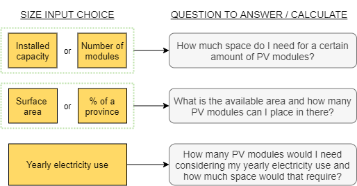
These area types relate to the following questions:
- What is the available area and how many PV modules can I place in there?
- How much space do I need for a certain amount of PV modules?
- How many PV modules would I need considering my yearly electricity use and how much space would that require?
When your PV system is large, it can happen that your PV system will generate more electricity than you would need. This we call overproduction.
Size input options
Often, the system size is calculated by means of how many PV modules fit in the available area. Though, in this tool the system size can be determined by specifying either the: installed capacity, the number of modules, the surface area, the yearly electricity use or (in case of field PV systems) the percentage of province.
Array layout
The so-called ‘PV array layout’ shows how many PV modules are placed in a row and how many rows
there are. In the design results, we show you one possible, simple array layout for your PV system design*.
What an optimal array for the PV modules in your PV system would be in real-life, depends on more detailed characteristics of your roof/field.
For example: the amount of roof-segments on which you want to place PV modules,
the obstacles on your roof, the safety-distance from the edges of the roof, shading by surrounding objects and the construction of your roof.
Creating a good ‘array layout’ (‘legplan’ in Dutch), can be done by for example letting a good installer examine the location on-site or remotely.
For a remotly designed array, advanced software tools are used.
Some of such tools are also freely online available. This PVP model currently focusses on the performance calculation of PV systems and does
not contain the functionality to design the PV array yourself.
*Read more about this calculated array layout here.
Overproduction?
When comparing the amount of PV modules that fit at your location and your yearly electricity use, we can find the following situations:
- Overproduction
There fit more modules on your roof/field than you would need. - Underproduction
There fit less modules on your roof/field than you would need. - Balanced production
The amount of modules that you need, fit exactly on your roof.
In case of overproduction you could do for example the following:
- Deliver the extra electricity back to the grid: this is not always profitable, since it depends on your situation and the current regulations regarding solar electricity production in your country.
- Use the extra electricity for electrical devices that substitute fuel-based devices: for example, induction cooking, an electric vehicle or an heat pump.
- Share the extra electricity with neighbors.
- Use part of the roof/field for a sun boiler instead of PV modules.
Installed capacity
The most common way of describing the size of a PV system is through its installed capacity. The capacity of a PV system is defined as its maximum potential to produce power. As power output is measured in Watt (W), the capacity unit of a PV system is Watt-peak (Wp). One kWp is a thousand Wp and a MWp a million. A typical PV module has an installed capacity of 270 Wp, though this can vary with the efficiency (η) and surface area (A) of the module, as shown in the equation below. GSTC is the sunlight intensity at which the panel is tested by manufacturers. The value of GSTC is 1000W/m2.

An example: a 1.6mm2 module with an efficiency of 18% will have a capacity of 288Wp. It is clear that when the efficiency or surface area of a module increases, the module capacity becomes larger.
The installed capacity only indicates the potential for electricity production. How much electricity will actually be produced by the system depends on many factors such as the location-specific weather during the year, the module orientation and on the electricity losses in the PV system.
Number of modules
The simplest way to size a PV system is to pick a certain number of modules for installation. Be aware that the installed capacity and the total surface area of the system may change a lot depending on the type of module you choose.
Surface area
Another way to determine the system size to choose is to look at the available area for installation. If the available installation area is limited, and the goal is to produce as much energy as possible on this surface, it makes sense to choose panels with the highest efficiency, as this is synonymous to capacity per unit area. Instead, if surface area is not the limiting factor, less efficient but cheaper modules could be chosen. A market-standard crystalline silicon module has a surface area of 1.63m2, while thin-film modules are usually smaller.
Yearly electricity use
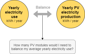
When you are interested to know how many PV modules you would need to balance (a part of) your average electricity use on a yearly base,
you can select this option. The PVP model then estimates what amount of PV modules is suitable in relation to your electricity use.
If you additionally would like to specify the available area, this can be done in the 'setup' tab. In this way, a comparison between the required number of modules and the available space can be made.
This tool in principle can only be used in case of a grid-connected PV system design. This means that a 100% load coverage does not automatically mean that you can be 'off-grid'. An off-grid PV system design is a complex issue. However, the total required number of modules as calculated from the yearly electricity use will be a good estimate for the minimum required system size for an off-grid PV system design.
Percentage of province
As an experiment, you can see what would happen if you cover an entire province, such as Utrecht, completely with solar panels.
Would the Netherlands be able to satisfy the national annual energy demand (3141 PJ, equivalent to 873 TWh [1]) with the amount
of solar energy produced? You can also play around with more realistic values, such as 3% of the total surface area available in the
province of your choice.
[1] CBS, Energiebalans; kerncijfers, 1946-2016, 2017.
System setup
While the sun moves throughout the day, the position of (most) PV systems is static.
Two important factors that determine the position of a solar module are tilt angle and azimuth angle.
The orientation of the PV modules is important since it influences the amount of sunlight energy that falls on the module
and thus the amount of electricity that it can produce.
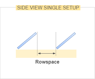
There are more factors that determine the setup of a PV system: rowspace, module orientation (landscape/portrait) and the geometry of your field/roof.
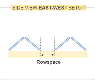
A special type of setup is a so-called 'east-west setup': here, part of the PV modules is facing towards the east and the other part towards the west (or similar opposite directions).
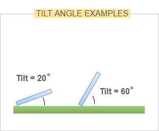
Tilt / Roof angle
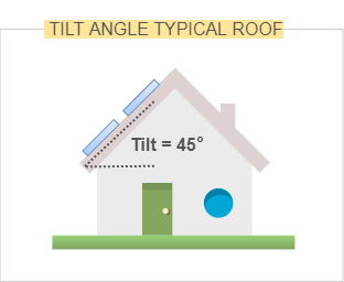
The tilt of a PV module is the angle between the solar module's surface and the Earth's surface. A module that is placed flat on the ground has a tilt of 0° (degrees).
A module that is placed vertically, for example on the wall of a building, has a tilt angle of 90°.
In the Netherlands, the optimal tilt angle is 37°, for modules that are facing towards the south.
At this tilt angle, the module receives the most amount of sunlight during a year.
Note that solar modules placed on a tilted rooftop usually have a tilt equal to the tilt of the rooftop.
Instead, PV modules that are placed on a flat roof or in a field are not restricted by the rooftop angle. The owner can decide which tilt angle to choose.
Azimuth / Roof orientation
The azimuth angle of a PV module is the direction that the front surface of the module is facing, measured in degrees relative to north. As a full circle is 360°, a module facing to the east will have an azimuth angle of 90°, south-facing modules have an azimuth of 180° and the azimuth of west-facing modules is 270°.
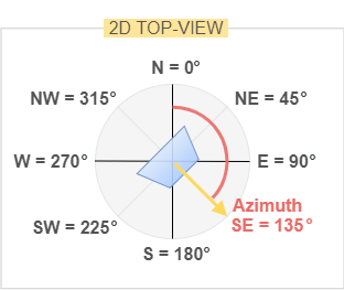
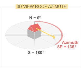
The irradiance energy from the Sun is largest when the Sun is at its highest point in the sky, which, in the Northern Hemisphere, occurs when the Sun is in the south. The optimal azimuth angle for the Netherlands therefore is 180°. As with tilt, the azimuth for a titled rooftop PV system is fixed by the azimuth of the rooftop itself. For PV systems on flat rooftops or field PV systems, the owner is free to decide the module azimuth.
Find the azimuth of your tilted roof
It is possible to find the azimuth of your rooftop using Google satellite images. You can do this yourself by following these simple steps.
- First, go to setcompass.com.
- Click on Draw Single Leg Route.
- Type your address in the Enter a place/postcode box at the top and click Submit.
- Click the
 Map icon in the top right, and select Satellite map.
 - Zoom in on your rooftop and then click Show compass in the top left corner.
- Place the compass center over the ridge on top of your house.
- Use the
 rotate icon to point the red arrow in a 90° with the ridge, in the direction of the southern rooftop side. In the top right corner the azimuth of your rooftop is shown.
 - Alternatively, you can rotate the arrow to point in the same direction as the ridge. In this case, to find your rooftop azimuth, look at the value in the top right corner. If it is larger than 180°, subtract 90° from the displayed value. If it is smaller than 180°, add 90° to the value. The new value is your rooftop azimuth. You can type this new value in the top right box and press enter to show the proper direction of the red arrow.

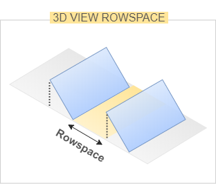
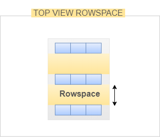
Rowspace
This is a factor only found in PV systems on a flat roof or in a field.
The distance between the modules (the rowspace) influences how much the module in the front can cast a shade on the module behind it.
The larger the rowspace, the less power will be lost due to this so called ‘mutual-shading’.
A good value for the rowspace typically is a tradeoff between available space and maximal power production.
Therefore, this optimal value also depends on the tilt angle of the PV modules. The smaller the tilt angle,
the closer the solar panels can be placed next to each other. As a rule-of-thumb we can say that a good rowspace value is:
30 degrees tilt --> 1,5 meter rowspace
20 degrees tilt --> 1,0 meter rowspace
10 degrees tilt --> 0,5 meter rowspace
When available space is not an issue, it is however recommended to place the modules at the smallest distance where no mutual shading occurs during the whole year. The longest shade during the year is found on the shortest day of the year, 21st of december, when the sun is in a very low position. This calculated minimal rowspace value depends of the location and the geometry of the system. In this situation, you can select the ‘No shading loss’ option and the PVP model will calculate the minimum rowspace needed to have no mutual shading loss during a year.
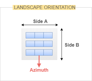
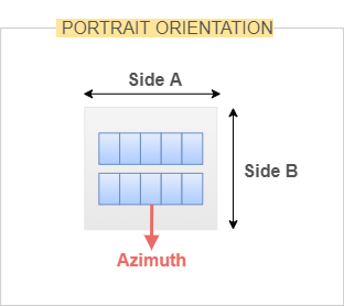
Module orientation
Does it matter if you place the PV modules portrait oriented or landscape?
For PV systems on tilted roofs, the main reason to choose for one or another is related to the shape of the roof and how to optimally make use of the
available space. Though, a landscape placement of the modules generally is a bit more difficult and demands slightly more mounting material.
For PV systems on a flat roof and for field PV systems, the orientation of the PV module additionally can influence the power output of your PV modules.
This is because in such systems, the modules can suffer from shading by the system itself (‘mutual shading’).
Different module technologies typically deal in a different way with such shading and thus the optimal orientation is related to the type of modules that you are using. In general, for PV systems where mutual shading occurs, crystalline-silicon PV modules perform better when placed in landscape mode and thin-film modules in portrait mode. Read more.
Area sides (optional input)
As mentioned, the size of your PV system can be determined in multiple ways. In some cases, it could be valuable to additionally specify the dimensions of your roof/field. In this way, it can be calculated whether the desired amount of PV modules would fit in the available area.
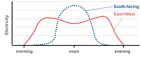
Eas-west setup
An east-west setup is a type of configuration for your PV modules where part of the modules is facing towards the east and the other part towards the west (or similar opposite directions).
While the total electricity production is slightly lower than in an optimally south-facing PV system, an east-west configuration can offer several advantages:
Energy production when it is needed the most
The electricity is produced more equally over the day (in comparison to a south-facing PV system).
The electricity is produced at times of the day when the electricity need is the highest: in the mornings and in the evenings.
Aligning the production with the consumption as much as possible could offer financial advantages when the regulations on net-metering change
in such a way that it will be more costly to deliver excess electricity back to the grid.
Cheaper mounting structure
In an east-west setup, the optimal tilt angle(s) of the modules is typically lower than in a south-facing system.
This lower tilt angle often results in cheaper mounting structures since they suffer less from strong-wind impacts.
Smart use of available space
The self-shading for an east-west setup is typically less of an issue, since the required minimal rowspace is now ‘filled’ with a PV module facing towards the opposite direction. In this way, more modules can be placed in the area. These ‘extra’ modules could compensate for the
slightly lower energy production due to non-south facing modules.
System components
The components of a PV system can be divided into two main categories:
(1) The PV modules (solar panels)
A device that can transform sunlight into usable electricity.
The PV modules are the central part of a photovoltaic system. It is a flat plate made of a semiconductor material that produces an electrical voltage when illuminated with sunlight.
(2) The Balance of System (BoS) components
All other components that are required for a working system.
Depending on the type of PV system, the most important BoS components are: mounting structure, wiring & cables, inverter, MPPT, a storage device and charge controllers.
In the PV system design tool, only the PV modules can be chosen by the user.
The BoS components are incorporated in the PVP model: cabling, an automatically selected inverter and an MPPT.
This means that this model will calculate the performance of grid-connected PV system designs.
PV modules
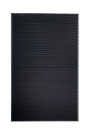
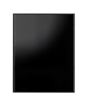
Currently, there are two main types of solar panels available on the commercial market: crystalline silicon panels and thin-film panels.
The division is based on the material properties of the semiconductor that a solar panel consists of.
In the current market, crystalline silicon panels take up >90% of the total production worldwide.
Within these two main types, module technologies differ on the type of material used and/or the structure of the panel,
which gives each technology unique attributes. The modules used in the PVP model were selected by choosing the standard module of a large solar panel manufacturer for each technology.
Important attributes of solar panels are, amongst others:
Efficiency:
The fraction of total sunlight energy that the module can convert to useable electrical energy.
Performance under high temperature:
As illuminated solar panels can heat up to temperatures of >70°, it is important that the panel still
performs well under high temperatures.
Manufacturing cost:
In general, modules with a high efficiency are also more complex to fabricate and therefore more expensive.
If the return on investment is most important for a PV system designer, it could be beneficial to choose a module with lower efficiency but also a lower price.
Inverter & MPPT
As all electrical equipment in households and the entire Dutch electricity grid require AC (alternating current) instead of DC (direct current) as an input,
the DC output of the PV panels must be converted to AC electricity. This is done with an inverter.
The PVP model uses a calculation method that automatically selects a suitable inverter from a database, depending on the input of your PV system design.
Cables
The choice of cables also influences the overall performance of a PV system. The cables should be chosen in such a way that the resistive losses are minimal. These losses depend on for example the material of the cables and their lenght and thickness. In the PVP model, the type of cables cannot be specified by the user. Instead, we use a fixed cable loss as explained here.
Cadmium telluride
Cadmium telluride (CdTe) is a thin-film technology. Of commercial thin-film technologies, CdTe is the only one that is able to achieve both a production cost and an efficiency that are comparable to the market-leading crystalline silicon technologies. An important disadvantage of CdTe is that telluride is a rare element, limiting the scale at which this technology could be applied worldwide.
CIGS
CIGS is an abbreviation of Copper, Indium, Gallium, and Selenide. CIGS modules consist of a mixture of these four elements. An important advantage of CIGS is its good performance under high temperature and during (partial) shading of the module. Disadvantages compared to CdTe and crystalline technologies are its lower efficiency and higher production costs.
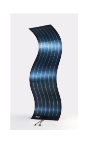
Flexible thin-film silicon
Thin-film silicon is the third thin-film technology. An important attribute of this technology is that it can be printed on a flexible material, and therefore placed on curved or other unconventional surfaces. A flexible thin-film silicon module can be much lighter than a conventional silicon module placed in a metal-glass frame. This makes the technology suitable for rooftops that are limited by the amount of weight that can be placed upon them. However, the efficiency of the technology is significantly lower than that of other thin-film or silicon technologies. In addition, the material is subject to light-induced degradation, which is a permanent reduction of the module efficiency due to exposure to light.
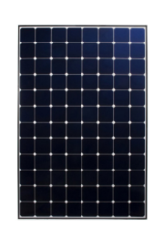
Heterojunction silicon
Heterojunction silicon is a specific structure which combines thin-film and monocrystalline silicon. The unique feature of this panel is that it 'sandwiches' a monocrystalline material in between two amorphous (thin-film) silicon layers, which reduces the amount of efficiency losses in the panel. Heterojunction panels achieve high efficiencies, but are also more expensive than the more common crystalline silicon panels.
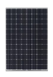
Monocrystalline silicon
Monocrystalline silicon panels are panels that consist of a layer of silicon with a single crystalline molecule structure. Monocrystalline panels achieve higher efficiencies than polycrystalline panels, albeit at a slightly higher manufacturing price. These modules boast some of the highest efficiencies in the commercial solar market while still being very affordable.
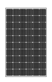
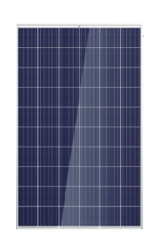
Polycrystalline silicon
Polycrystalline silicon panels consist of multiple silicon crystals. The panels are easy and cheap to fabricate, whilst still achieving efficiencies comparable to (but below) those of monocrystalline panels. Due to the extremely low production cost, polycrystalline panels take up the largest market share in the commercial solar panel production.
System performance
The performance of a photovoltaic system can be expressed in a number of manners.
Primarily, the power* or energy** output of the system is an indicator of its performance.
While this total system power production is a useful value to determine the contribution that it can make to the demand of a household (or a region in case of large-scale systems), additional performance indicators for PV systems are used to compare the performance of different systems.
The Dutch PVP model calculates and displays three of the most common indicators: energy yield, performance ratio, and system efficiency.
*Power is expressed in Watts (W), which is the energy
production or consumption per unit of time. A television, for example, may have a power demand of 50W, which means that it consumes 50 Joules of
energy per second (J/s).
**Energy is expressed in Watt-hours (Wh), which is the total energy production or consumption in a given period.
It is found by multiplying the power output by the duration of the power output of the system. For example, if the TV runs for 4 hours,
the amount of Wh of energy consumed will be 4*50=200Wh. An average Dutch household consumes 2910kWh per year, i.e. around 8000Wh per day.
On average, a PV system should be able to produce the same amount of electricity per day to make the household self-sufficient.
Naturally, the daily energy production in winter will be lower than in summer.
Energy Yield
Energy yield (EY) is a performance indicator that allows for comparison between systems of different sizes. It is calculated by dividing the annual system energy production (in kWh) by the installed capacity (in kWp) of the system, and has a unit of kWh/kWp. The EY is strongly dependent on the amount of available sunlight, and is therefore location-dependent. A specific PV system design will have a much higher EY when placed in Dubai than if the same system were placed in Oslo.
Performance Ratio
Performance ratio (PR) indicates the amount of energy or power losses occurring in a PV system. A PR of 90% indicates that 10% of the maximum
available electricity is lost in the power conversion and transport processes in the PV system. The PR is a highly useful tool for comparing the
performance of PV systems as it takes the effect of system size and available sunlight out of the equation. The PR therefore allows for comparison
between systems of different sizes and of different locations.
The PR is the ratio of hours of peak power production to the hours of peak sunlight available. The EY is equivalent to the hours of peak production:
how many hours in the year has the PV system been able to achieve its peak installed capacity? The number of hours of peak sunlight available is
calculated by dividing the annual sunlight energy on the panels (in kWh/m2) by the sunlight power intensity under standard test conditions (STC),
which is 1000W/m2 (comparable to the intensity of sunlight on your face on a bright summer day in the Netherlands).
Manufacturers determine the output power (i.e. installed capacity) of PV panels under STC, which also includes the requirement that module
temperature must be 25°C, which is achieved through short measurement times or artificial cooling. In real-life conditions, module temperatures under
a 1000W/m2 illumination will be far higher than 25°C, leading to a reduction in module performance,
i.e. a lower power output than the installed capacity.
The reasoning behind the PR is then as follows: in reality, energy losses will occur in the PV system that do not take place in the 'ideal'
measurement of the panel performance under STC. All these energy losses together can then be indicated by the PR of a system, where a PR of
100% would mean that the PV system would operate at STC performance levels. In real-life operations, rooftop systems commonly have a PR of
70-80% while large-scale field systems that are well-maintained can have PR values of 80-90%. The PR is calculated according to the formula below.
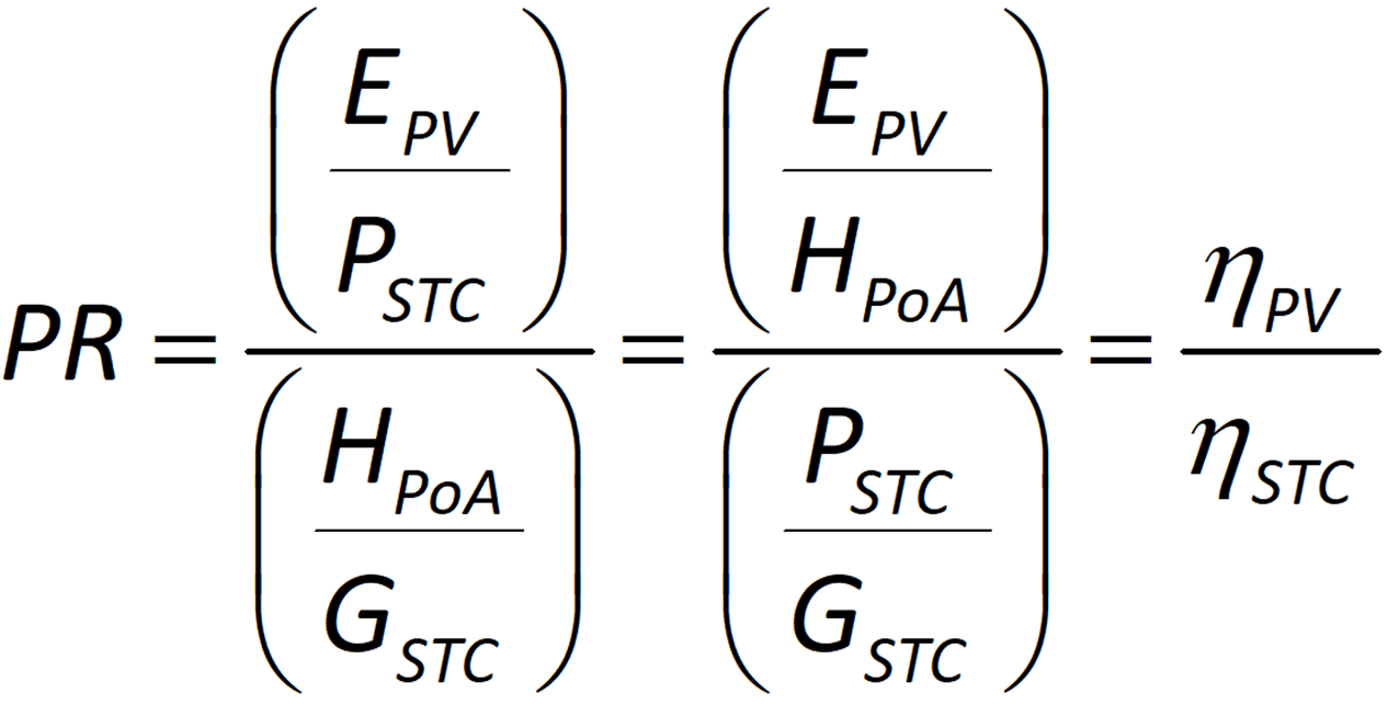
In which EPV is the system energy production (both the DC- and AC-side production can be used), PSTC is the installed capacity, HPoA is the plane-of-array irradiation, GSTC is the STC irradiance of 1000 W/m2, ηPV is the final system efficiency, and ηSTC is the panel efficiency under STC (the 'ideal' efficiency).
System efficiency
The PV system efficiency shows how much of the available sunlight energy that falls on the PV panels is ultimately
converted into useable electricity by the PV system: the sunlight-to-electricity conversion efficiency.
The PV system efficiency depends many factors, as further explained here.
In general, annual PV system efficiencies of 17% are quite impressive.
Efficiency / Losses
The process of creating electricity from sunlight involves multiple energy-conversion steps. In each step, a part of the energy from the
incident sunlight is lost. Energy losses can also be expressed as an efficiency*.
While often only the STC efficiency of a PV module is noted, it is interesting to look at the efficiency of the whole PV system. So what determines this overal system efficiency? These are:
- The theoretical maximum efficiency of a solar cell:
This is a limit around 30% (for single-junction solar cells) - The design & material of the solar cell and the PV module:
This results in the (fixed) STC efficiency of the PV module. This ηSTC strongly depends on the material used: mono-Si panels commonly have a higher efficiency than thin-film panels, for example. - The dynamic surroundings of the PV module:
Due to changing weather, shading patterns, dust etc, the efficiency is in fact not a fixed value, but it changes over time. - The setup of the PV modules:
The tilt, orientation etc. - All other components in a PV system:
Balance of System (BoS) components such as inverters, cables, MPPT etc.
*A 20% energy loss means an energy efficiency of 80% (=100%-20%).
The PV system efficiency is the final electrical energy output divided by the sunlight energy input. This efficiency is always lower than 100%.
The efficiency breakdown graph
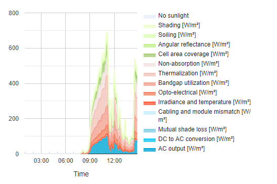
The efficiency graph created by the PVP model (see example figure below) displays the calculated efficiency losses that would occur today for your designed PV system.
You will see that this graph will look different each day, strongly depending on the weather conditions. We can divide the losses into three main categories: light capture losses, PV module conversion losses and Balance of System (BoS) losses. After subtracting all these losses, the final AC electricity output that can be used by your devices remains (blue area in the graph).
You can also view the performance values when light capture losses (soiling, reflectance and shading by surroundings) are excluded: to do so, click on the switch in the overview. This is interesting when you have for example a rooftop PV system without any obstacles in the nearby surroundings.
Light capture losses
Light capture losses are the losses in sunlight energy before the light is absorbed by the solar panel. This category involves losses caused by shading by surroundings, soiling, angular reflectance loss and cell area coverage.
Shading by surroundings
Shading refers to the blocking of sunlight by surrounding objects. This can be other buildings, trees, chimneys, etc.
The PVP model assumes a 6.88% annual shading loss for rooftop PV systems, and 0% for field PV systems.
Naturally, the shading loss will be different for each individual rooftop. A location-specific shading analysis,
based on geographic height data combined with a Sun position calculator, is offered by multiple commercial PV system modelling software companies,
such as Solar Monkey.
For field PV systems and PV systems on flat roofs, another type of shading loss is considered: mutual-shading loss.
In the PVP model, this loss is not treated as a light capture loss, but as a BoS component loss.
Soiling
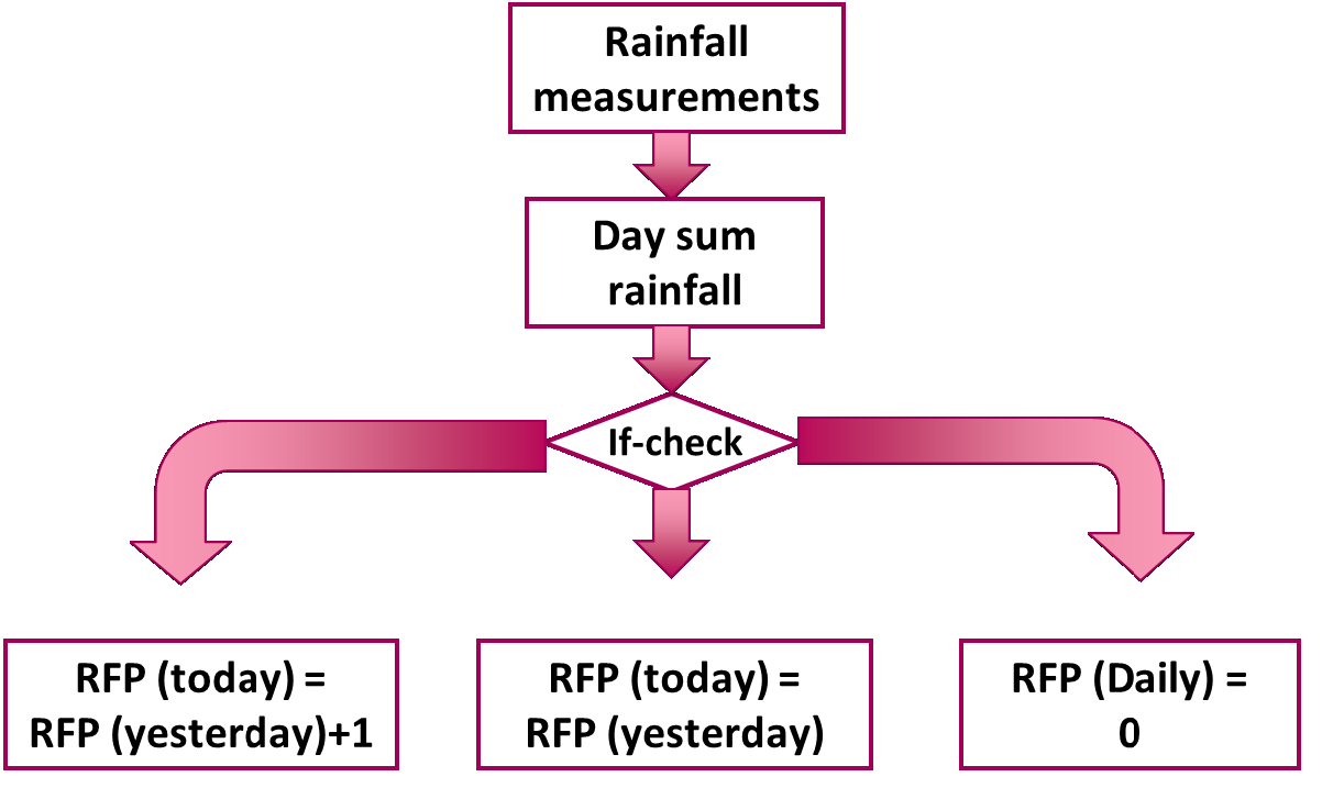
Soiling is the efficiency loss that occurs due to the absorption or reflection of light by dust or dirt that has accumulated on the panel. The amount of soiling loss is related to the number of days without significant rainfall (the rain-free period, RFP), as rain is able to clean the dust of the panel and 'reset' the soiling loss to 0.
AOI reflectance
Angular reflectance refers to the additional light reflectance from the module's surface, due to non-perpendicular incidence of sunlight on a module's surface compared to perpendicular light incidence. In compliance with Snell's law, the smaller the angle between the modules's surface and the direction of the sunlight, the larger the reflectance. The PVP model uses a fixed angular reflectance factor of 4%, based on [1].
Cell area coverage
Only a part of the panel surface consists of photoactive solar cells that can generate power. The rest of the module area consists of space between the cells and the frame of the module. The light falling on this inactive area cannot be converted to electricity. Therefore, to calculate the size of this light capture loss, the area coverage ratio of photovoltaically active to total module area needs to be calculated based on the dimensions given by the manufacturer. The total loss differs between panel types, but losses are in the range of 7-14%.
PV conversion losses
When a PV module is illuminated, it can generate an electrical current. The power loss that occurs inside of the PV module material during this
process can be separated in two parts:
STC module efficiency:
The efficiency for PV modules in datasheets is given as a fixed percentage: this percentage is the so-called STC efficiency:
the efficiency of the PV module under Standard Test Conditions.
Theoretical efficiency losses: the conversion efficiency of a PV module has a theoretical limit of around 30%, due to the spectrum of the incident sunlight
and the material properties of the solar cells*. This is determined by processes such as non-absorption, thermalization and bandgap utilization.
Read more about it here.
Opto-electrical losses: these losses are related to how well the solar cell is designed.
The better the design of the solar cell, the closer the efficiency of the PV module reaches its theoretical efficiency limit.
It is a challenge for researchers and manufacturers to reduce the size of two types of losses: optical losses (referring to the fact that not all
photons with above-bandgap energies are absorbed), and electrical losses (referring to the fact that not all the electrical energy generated from
absorbed photons is collected at the electrodes of the solar panel). Together, these imperfect solar cell losses are referred to as
opto-electrical losses. A precise characterization of the opto-electrical losses in the various module technologies is complex,
but the size of the opto-electrical losses is equivalent to the difference between the theoretical efficiency of a material
and the efficiency of a panel of this material as measured by the manufacturer (ηSTC).
*This may sound low, but to put it into perspective, consider that the sunlight-to-energy conversion efficiency of fossil fuels is miniscule in comparison: the photosynthesis of plants converting sunlight to chemical energy is already a very inefficient process. In the decomposition and fossilization of dead biomass a large portion of this chemical energy is lost. In addition, the formation of fossil fuels takes place over millions of years. By comparison, the instantaneous conversion of sunlight to electricity in a PV system is a much more efficient and straightforward method of utilizing the Sun's energy.
BoS losses
These BoS losses are the losses that occur in the PV system components other than the PV modules. In the PVP model we consider (DC) cabling and module mismatch losses and DC to AC conversion losses: inverter & MPPT losses. Additionally, for flat roof and field PV systems, mutual shading loss is considered.
Cabling and mismatch
Module mismatch losses occur when modules in a string (a series connection of modules) produce different currents which leads to power dissipation in the module string, while Ohmic cabling losses are due to the electrical resistance of the cable wires when transporting current. Module mismatch losses are estimated at 1.5% and Ohmic cabling losses at 0.5% in the PVP model [1].
Inverter & MPPT
The PVP model calculates the inverter efficiency based on the inverter capacity and the power input into the inverter at a given moment in time,
using the Sandia National Laboratory inverter model [1]. The efficiency of an inverter is low when the input power produced by the PV modules is
far below the inverter input capacity. This means that inverter losses are high in the winter and at the start and end of the day (low light conditions).
The PVP model also includes a 3.15% efficiency loss due to maximum power point tracking (MPPT), an algorithm commonly
built in to inverters to ensure that PV panels work at the voltage and current point that will result in the maximum power output [2].
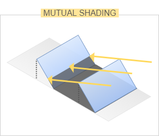
Mutual shading
In this tool, two types of shading are distinguished: ’shading by surroundings’ and ’shading by the system itself’. The latter happens in field PV systems or in systems on flat roofs and is referred to as ’mutual shading’. Mutual shading loss is modelled as a DC power loss: this loss represents the DC power that is lost due to self-shading of the PV modules. It is calculated as the difference between what the DC power output would be when no mutual shading occurs and what it would be when part of the modules is shaded. Details of this approach can be found here.
Economics
Your system design choices are used to calculate the total system costs (investment).
The calculated annual energy production is used to calculate the total annual revenue.
Your design choices determine the assumed economic input values that are used for these calculations.
It is important to note that these financial calculations are estimates, since they are based on many economic assumptions.
For example, in case of overproduction, the excess electricity could be sold back to the grid (net-metering).
Whether this is profitable relates to the price of the electricity and the discount rate.
In addition, four economic indicators that are relevant for PV systems are calculated to determine whether the investment is worthwhile:
the net present value (NPV), the (discounted) payback period ((D)PBP), the compound annual growth rate (CAGR),
and the levelized cost of electricity (LCoE). Each indicator can highlight a different aspect of the investment.
Read more about the economic calculations here.
Discount rate
The discount rate is a concept that is related to the time value of money.
As money can accumulate value through interest, it is more beneficial to have a certain amount of money now than the same amount at
a moment in the future. When translating future gains or losses in money to current-day values, the discount rate is used.
The discount rate can be seen as a standard interest rate for the investment.
As an example, a €105 gain one year from now would be equivalent to a €100 gain right now at a discount rate of 5%.
Therefore, the higher the discount rate, the higher future gains must be for the investment to be profitable compared to a standard investment
at the given discount rate.
Two scenarios, one with a low discount rate of 3%, and one with a high discount rate of 7%, have been calculated in the PVP model
to exemplify this influence. If a PV system investment is profitable at a certain discount rate, this means that it is a better investment
opportunity than another investment with an interest rate equivalent to the discount rate.
The low discount rate and high discount rate scenarios are therefore mostly interesting in comparing an investment in a PV system to another
investment opportunity at the given discount rate, and are therefore mostly used by financial investors.
For most households or individuals that would otherwise keep their money on the bank at a 0-1% interest rate, the economic factors most relevant
to them are the non-discounted values.
Net-metering
The PV system electricity is not always in balance with your electricity use. This means that when the production exceeds the use (overproduction),
the excess solar electricity is delivered back to the grid. When the electricity use is higher than the production, electricity is taken from the grid.
At the end of the year (in the Netherlands), a comparison is made between the amount of electricity delivered to,
and the amount taken from the grid. The delivered electricity is substracted from the token electricy, and you will only pay for the remaining kWh.
This is called 'net-metering'. This very beneficial regulation will remain untill 2023. Note that there is a net-metering limit and that
when the yearly delivering to the grid exceeds the electricity taken from the grid, the amount of money you get depends on your electricy company.
A clear description on net-metering is found here.
Economic indicators
Net present value
The NPV of a system represents the final profit that would be made over the entire system lifetime if one were to invest in it.
It follows that a positive NPV represents a good investment whereas a negative NPV is a bad investment.
Note that when a discount rate is applied, the system can still be profitable, i.e. provide the investor with more money than he initially invested.
A negative discounted NPV, however, does indicate that the net profit would be less than the investor could receive from an alternative investment
at the given discount/interest rate.
Payback period
For PV systems, the lifetime of the system is currently estimated at 25 years by module manufacturers.
As a PV system requires a high initial investment which is earned back through electricity savings and sales, the investment must be earned back
in 25 years. Therefore, a PBP of less than 25 years indicates a good investment. Every year after the PBP contributes to the net profit of the system.
Compound annual growth rate
The CAGR describes the average interest made over the total investment considering the total revenue made on the system over its lifetime.
The value of CAGR can be used for comparisons with interest rates of alternative investments.
Levelized cost of electricity
The LCoE is an important parameter when comparing the production costs of different electricity sources.
It represents the amount of money it costs to produce one kWh of electricity, and therefore LCoE is expressed in €/kWh.
Comparing the LCoE of solar energy to that of conventional (fossil) electricity sources can show whether photovoltaics are economically
competitive with these sources.
Local weather & climate
Website visitors can choose any location in the Netherlands using the Google map.
This location (address) then deterimines from which KNMI weather station the meteorological data is obtained.
The exact location is also used for calculating the position of the sun during the day (and year).
The meteorological data serves as input for the irradiance models that finally calculate the plane of array irradiance (GPoA).
After determining the GPoA, several irradiance (light capture) losses are substracted.
KNMI data
The KNMI has provided the TU Delft with access to real-time instantaneous weather measurements with a time resolution of 10 minutes,
which are not publically available. The data are gathered every 10 minutes from 46 onshore weather stations throughout the country.
To create annual climate datasets, hourly KNMI station measurements were downloaded for the period of 1991-2017 for each of the 46 stations and then edited as explained here.
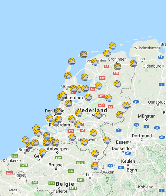
A map of the KNMI stations used in the PVP database is shown in Figure 1. More information on each of the weather stations can be found here. Website users can view and download the data of any of the 46 stations. They can also do this for each of the 12 Dutch provinces, of which the data are the mean values of all weather stations located in that province.
Fig. 1 - Map of KNMI weather stations providing measurements stored in the PVP database. The KNMI station code and station name are displayed when an icon is clicked.
The following real-time meteorological parameters* used to simulate PV system performance are stored in the PVP database:
- Global horizontal irradiance [W/m2]
- Ambient temperature [°C]
- Ground temperature [°C]
- Wind speed [m/s]
- Cloud coverage [okta]. A cloud coverage of 1 okta means that one-eighth of the entire sky is covered by clouds.
- Atmospheric pressure [Pa]
- Rainfall [mm/hr]
*Measurements are not precisely available instantaneously. There is in fact a 10-40 minute time difference between the current time and the time of measurement, due to the delay in data transfer from the weather stations to the KNMI database. The relevance of these measurements to the performance of PV modules is explained here.
Meteorological databases
For construction of the PVP climate database, hourly KNMI station measurements were downloaded [1] for the period of 1991-2017 for each of the 46 stations and then averaged for every hour between years to one climate dataset of 8784 hours ((365 days + 1 leap day)*24 hours). An example of such averaging, in this case for wind speed, is shown in Figure 1.
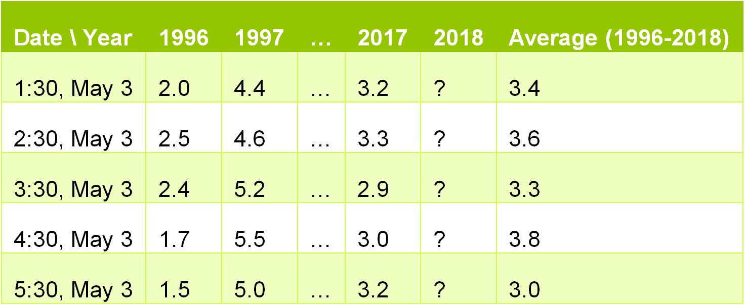
Fig. 1
An unique feature of the PVP model, is that the climate database is dynamically updated. Every hour, the hourly average of the real-time
weather measurements is added to the climate database by making a weighted average with the climate parameter values in the historical database.
The advantage of this feature is that every new weather measurement contributes to a more accurate estimate of the local climate.
This feature allows developments like climate change to be incorporated into the datasets used by the PVP model,
unlike static datasets that are only representative for a certain period in time, such as 2005-2010. A flowchart of the procedure performed every hour
to update the historical climate database is shown in Figure 2.
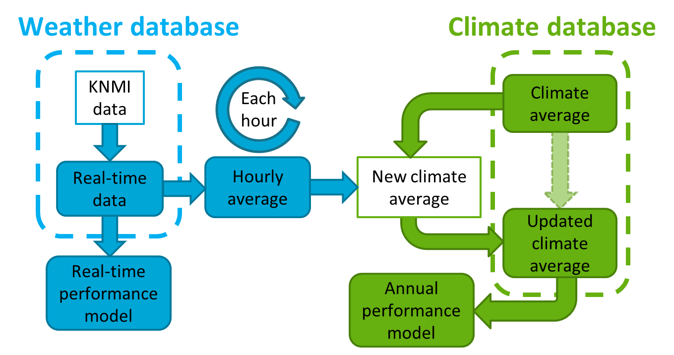
Fig. 2 - Connection between the real-time and climate database. The creation of a weighted average of the new and historical measurements allows the annual dataset to become dynamic.
[1] Koninklijk Nederlands Meteorologisch Instituut (KNMI), KNMI Data Centre, 2018.
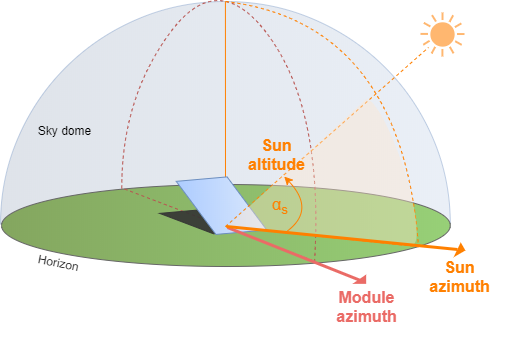
Sun position
The position of the sun at a certain location at any time of the day can be calculated mathematically, expressed as an sun altitude (αs) and sun azimuth. The model used for this calculation is described in detail in chapter 18 of [1].
Irradiance models
The performance of a PV system is highly dependent on the relative position between the sun and the PV modules,
as well as on the characteristics of the sunlight: the irradiance components and how the sunlight reaches the surface of the PV module.
These factors need to be evaluated for the time and day of the year as well as for the specific location coordinates.
We can distinct three irradiance components: direct, diffuse and reflected (albedo) sunlight.
First, the irradiance components on a horizontal surface are calculated. Then, the effective radiation striking the module surface
is calculated as the component of the solar radiation that reaches the Plane of Array (GPOA).
Horizontal surface irradiance
Based on the measured global radiation on the ground, a model has been implemented that extrapolates the direct and diffuse (horizontal) irradiance components. The model has been developed by Reindl et al. [1] and makes use of a mathematical step function that calculates the diffuse fraction of solar radiation according to the value of the clearness index. This mathematical correlation is valid for northern European locations at latitudes of approximately 50-60°N.
The clearness index measures the attenuation of incoming solar radiation due to the atmosphere. It is therefore defined as the ratio of the horizontal global irradiance on the ground (Gglobal) to the corresponding incident irradiance from the atmosphere.
Tilted surface irradiance
The effective radiation striking the module surface has been calculated as the component of the solar radiation that reaches the Plane of Array (GPOA). This component has been approximated as the sum of a direct beam (Gbeam), a reflected beam from the ground (Greflected) and the fraction of the horizontal diffused light that reaches the module (GdiffusePOA).
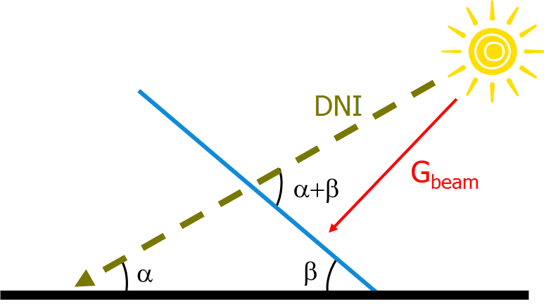
Fig. 1 - Beam component of the incident solar radiation on the modules surface
For the direct normal irradiance (DNI), the direct beam has been derived by considering the relative angle between the module surface and the direction of the sunlight (Figure 1), as:

Where β corresponds to the module tilt angle; α and As are the instantaneous elevation and azimuth of the sun respectively, and Am is the azimuth/orientation of the modules. More specific details on how to calculate the instantaneous position of the sun can be found in [1].
The radiation reflected from the ground (Greflected) is calculated by considering the reflectivity of the ground surface and the tilt angle of the modules [2].
The diffuse radiation that reaches the modules is also calculated using a model developed by Reindl et al. This consists of an anisotropic diffuse model that considers the threefold effect of isotropic, circumsolar and horizon brightening components of the diffuse radiation on the module surface [3].
The sum of these three components determines the total amount of solar energy instantaneously available at the module surface.
[2] Sandia National Laboratories Plane of Array - Ground reflected radiation, 2014.
[3] Reindl D.T. et al., Evaluation of hourly tilted surface radiation models, Solar Energy Journal, 1990.
Light capture losses
A part from the irradiance incident on the module surface is lost due to soiling, shading and reflection.
These so-called light capture losses are thus losses in sunlight energy before the light is absorbed by the solar panel.
There exist several modeling approaches each differing in how to deal with such losses. A tradeoff between calculation speed and accuracy was made
when deciding on a suitable approach for the PVP model.
These light capture losses are incorporated in the form of an efficiency chain:
𝐺𝑃𝑜𝐴,𝑓𝑖𝑛𝑎𝑙 = 𝐺𝑃𝑜𝐴,𝑝𝑟𝑖𝑚 ⋅ 𝜂𝑠𝑜𝑖𝑙𝑖𝑛𝑔 ⋅ 𝜂𝑠ℎ𝑎𝑑𝑖𝑛𝑔 ⋅ 𝜂𝑟𝑒𝑓𝑙𝑒𝑐𝑡𝑎𝑛𝑐𝑒
Shading
The PVP model assumes a 6.88% annual energy loss for rooftop PV systems due to shading by surrounding objects. This loss value is based on shading simulations of 5400 PV systems by the PV system modelling company Solar Monkey. In this case, 𝜂𝑠ℎ𝑎𝑑𝑖𝑛𝑔 = 0.9312.
For field PV systems, a 0% shading loss (𝜂𝑠ℎ𝑎𝑑𝑖𝑛𝑔 = 0) is assumed as these systems are usually placed in a ‘free-horizon’ location (no surrounding obstacles).
For field PV systems and PV systems on flat roofs, another type of shading loss is considered: mutual-shading loss. In the PVP model, this loss is not treated as a light capture loss, but as a DC power loss.
Soiling
Soiling is the efficiency loss that occurs due to the absorption or reflection of light by dust or dirt that has accumulated on the panel. The amount of soiling loss is related to the number of days without significant rainfall (the rain-free period, RFP), as rain is able to clean the dust of the panel and 'reset' the soiling loss to 0.
The PVP model assumes a 2 mm/day rainfall to be enough to completely clean the panel [1]. The soiling loss increases by 0.083%/day (the soiling factor, SF) for each day with less than 2 mm rainfall [1]. The PVP model uses real-time KNMI rainfall measurements to track the RFP for each location in the Netherlands. The soiling efficiency is then finally expressed as: 𝜂𝑠𝑜𝑖𝑙𝑖𝑛𝑔 = 1 − (𝑅𝐹𝑃 ∙ 𝑆𝐹).
AOI reflectance
Angular reflectance refers to the additional light reflectance from the module's surface, due to non-perpendicular incidence of sunlight on a module's surface compared to perpendicular light incidence. In compliance with Snell's law, the smaller the angle between the modules's surface and the direction of the sunlight, the larger the reflectance. The PVP model uses a fixed angular reflectance factor of 4%, based on [1].
Cell area coverage
Only part of the panel surface consists of photoactive solar cells that can generate power. The rest of the module area consists of space between the cells and the frame of the module. The light falling on this inactive area cannot be converted to electricity. Therefore, to calculate the size of this light capture loss, the area coverage ratio of photovoltaically active to total module area needs to be calculated based on the dimensions given by the manufacturer. The total loss differs between panel types, but losses are in the range of 7-14%.
DC module efficiency
The efficiency of a PV module is influenced by both the module temperature and the level of incident radiation. Both are related to the constantly changing weather conditions. For finding the temperature of the module, a so-called fluid-dynamic model is used. The incident irradiance is calculated as described here. Once the irradiance on the module and the temperature of the module have been calculated, the effect of this on the efficiency of the module itself can be calculated.
Fluid-dynamic model
The approach of this model is a thermal energy balance between the module and the surrounding environment [1] (Figure 1), to determine the temperature of the module depending on the weather conditions. The model also takes into account the effect of the mounting configuration of the operative PV system. The energy balance performed is also referred as the 'fluid-dynamic model', since the air flow regime around the module is a key parameter for determining the operative module temperature.
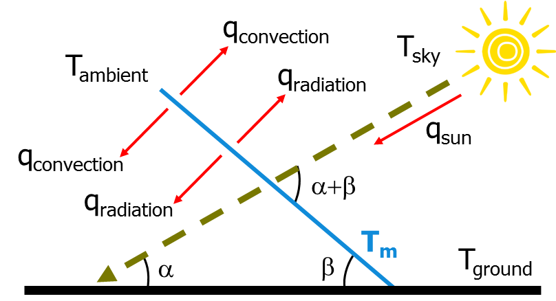
Fig. 1 - How a PV module exchanges heat with the surrounding environment.
To perform the energy balance, the PV module is modelled as a single uniform mass at a temperature Tm. The modes of heat transfer between the module and the surroundings are respectively:
- heat received from the sun in the form of insolation (qsun).
- convective heat exchange with surrounding air at the front and rear side of the module (qconvection).
- radiative heat exchange between the front surface and the sky and between the rear surface and the ground (qradiation).
A uniform module temperature throughout each layer has been considered due to the low thickness of the active layer of the cell with respect to the entire cell assembly, together with the low heat capacity of the cell material compared with the other layers [2]. A steady state approximation has also been performed due to the relatively long (10 minute) time interval between one series of data and the following series [2]. The module operative temperature has been calculated by performing an iterative process for each set of parameters received.
Knowing the incident radiation on the module surfaces and their operative temperatures; real-time module efficiency and specific power output [W/m²] can be calculated by separately assessing the effect of temperature and incident irradiance [3].
[2] Jones A.D. and Underwood C.P., A thermal model for photovoltaic systems, Solar Energy Journal, 2001.
[3] Lorenz E., et al., Regional PV power prediction for improved grid integration - Progress in Photovoltaics: Research and Applications, 2011.
Temperature / irradiance effects
Once the irradiance on the module and the temperature of the module have been calculated, the efficiency of the PV conversion itself can be calculated. Irradiance values lower than 1000W/m², which is the irradiance at which the manufacturer tests the standard efficiency of each module, will lead to lower panel efficiencies. Temperatures above 25°C, again the standard test condition module temperature, will lead to a decrease in module efficiency. Incorporating both these effects allows for calculation of the DC module efficiency.
As the module efficiency is tested at a specific irradiance intensity and a specific module temperature (the standard test conditions, STC), any deviation from this irradiance and temperature will affect the module efficiency. In general, the PVP model takes a logarithmic positive relation between irradiance intensity and efficiency: the higher the irradiance, the higher the module efficiency. Conversely, there is a linear inverse relation between module temperature and efficiency. The higher the temperature, the lower the conversion efficiency [1].
PV conversion losses
For the means of creating a figure that displays the breakdown of all losses occuring in the PV system, the theoretical and opto-electrical losses within the PV module are further categorised*. This involves the processes of non-absorption, thermalization, and bandgap utilization. These losses are inherent to photovoltaic materials and their sizes can be calculated based on the material properties. They therefore determine the theoretical efficiency limit of a specific photovoltaic material. For silicon, a theoretical limit of 29.43% is estimated (i.e. an ideal crystalline silicon cell could convert 29.43% of sunlight energy to electricity) [1].
The calculated values of these losses are only used to display in the efficiency breakdown figure. Read here how these calculations are done. For the yield calculations, the PV conversion losses are calculated by using the STC efficiency corrected by the temperature and irradiance effects as described here and here.
Non-absorption
Once the light has entered the panel, the energy can be absorbed by the panel material. To understand this process, light can be seen as a collection of energy packages called photons. Each photon can have a frequency which is proportional to its photon energy. The higher the frequency, the higher the energy of the photon.
To be absorbed and be able to free an electron (an electrical charge carrier) in the photovoltaic material, a photon should have an energy higher than the 'bandgap energy', a photovoltaic material property. All photons with an energy below the bandgap energy pass through the panel without being absorbed. The energy contained in these photons contribute to the non-absorption loss.
Thermalization
An electron freed by a photon of sufficient energy is only able to contain the bandgap energy, but no more. Therefore the photon energy minus the bandgap energy (a photon's excess energy) is lost as heat in the module in a process called thermalization.
Bandgap utilization
In solar cells operating above zero Kelvin (the absolute freezing point at -273.15 °C), the module is in thermal equilibrium with the environment and therefore recombination processes take place, in which electrons fall back to their original energy level and emit a photon again. The loss of energy due to recombination of charge carriers leads to less of the bandgap energy being used, i.e. an additional loss called bandgap utilization loss.
Opto-electrical
In reality, solar cells are not ideal, and it is a challenge for researchers and manufacturers to reduce the size of two types of losses: optical losses (referring to the fact that not all photons with above-bandgap energies are absorbed), and electrical losses (referring to the fact that not all the electrical energy generated from absorbed photons is collected at the electrodes of the solar panel). Together these imperfect solar cell losses are referred to as opto-electrical losses.
A precise characterization of the opto-electrical losses in the various module technologies is complex, but the size of the opto-electrical losses is calculated as the difference between the theoretical efficiency of a material and the efficiency of a panel of this material as measured by the manufacturer.
BoS components
In the PV system design tool, only the PV modules can be chosen by the user. The BoS components are incorporated in the PVP model: cabling, an automatically selected inverter and an MPPT. This means that this model will calculate the performance of grid-connected PV system designs.
Cables & mismatch
Module mismatch losses occur when modules in a string (a series connection of modules) produce different currents which leads to power dissipation in the module string, while Ohmic cabling losses are due to the electrical resistance of the cable wires when transporting current. Module mismatch losses are estimated at 1.5% and Ohmic cabling losses at 0.5% in the PVP model [1].
Inverter
The PVP model uses a calculation method that automatically selects a suitable inverter from a database (based on the SNL database [1]). This selection procedures depends on the input of your PV system design. The PVP model calculates the inverter efficiency based on the inverter capacity and the power input into the inverter at a given moment in time, using the Sandia National Laboratory inverter model [1].
The flowchart below shows a schematic overview of how the inverter selection, topology and efficiency is determined. For a detailed explanation is referred to [2].
MPPT
Also incorporated into the final DC to AC conversion efficiency is the Maximum Power Point Tracker (MPPT) efficiency. The MPPT is a device that allows the solar panel to operate at the voltage and current that gives the largest power output at that moment. The MPPT efficiency is stable and high. In the PVP model ηMPPT is assumed to be 96.85% [1].
Inverter selection
The three considered topologies are a ’central inverter’, a ’team inverter’ and a ’string inverter’, corresponding to the chosen total installed PV capacity. The inverter selection process is based on two criteria:
- (1) The nominal inverter input power must be close to the nominal installed capacity of the module string and not exceed this;
- (2) The selfconsumption of the inverter should be as low as possible.
The required minimum inverter power depends on the determined type of inverter and its corresponing assumed number of subsystems (NoS).
In the PVP model, NoS equals 1 in case of a central inverter and 4 in case of the team inverter.
Though, for a string inverter, the number of subsystems initially is unknown. In this case the starting point is a variety of possible stringlengths: 12, 14, 16, 18 or 20 modules per string.
A forloop is used to loop through all inverters from the database searching for the inverter which best matches the criteria (1) and (2).
For each type, the required inverter power is downscaled with the Inverter Sizing Factor* (ISF).
This Inverter Sizing Factor is a tilt- and azimuth-dependent factor used from the research of [1].
Inverter topology
As input for the efficiency calculations, it is needed to determine the topology of the inverter: the number of modules in a string (series) and the number of strings (parallel) for the subsystems. For each inverter topology, the maximum inverter string-length is defined by the input voltage of the inverter.
We compare the nominal inverter voltage with the average maximum power point voltage of the system to estimate the maximum number of modules
connected in a string.
The calculated number of modules connected in series, 𝑁𝑠, in a subsystem is then set to be one of the following three options: (1) 𝑁𝑠 = 𝑁𝑠,𝑚𝑎𝑥, (2) 𝑁𝑠 = 1 or (3) 𝑁𝑠 = 𝑁𝑠𝑢𝑏𝑠𝑦𝑠𝑡𝑒𝑚.
It is preferable to connect as many modules as possible in series, option (1), since this lowers the
currents on the DC side, resulting in less cable losses.
Inverter efficiency
The PVP model calculates the inverter efficiency based on the inverter capacity and the power input into the inverter at a given moment in time, according to the Sandia National Laboratory inverter model [1]. The efficiency of an inverter is low when the input power produced by the PV modules is far below the inverter input capacity. This means that inverter losses are high in the winter and at the start and end of the day (low light conditions).
Additional to the parameters from the inverter database, the DC power input and
voltage to the inverter is needed. Both depend on the determined topology of the inverter.
The DC input voltage equals the total voltage of a subsystem string, calculated by multiplying the DC
voltage of one module with the number of modules in the string. The DC power input depends on the
actual DC power output of one module and the number of modules in a subsystem.
In the team inverter topology, the total DC system power can be divided over the four inverters in the
most efficient way. In case of a low power production per subsystem, the amount of active inverters
can be reduced, increasing the overall conversion efficiency.
Due to the model being less accurate in case of very low voltages, an additional check is implemented
to ensure that the efficiency cannot exceed 100%.
Mutual shading loss
The mutual shade loss calculation model is developed within the PVMD group of the TU Delft, as read in [1] . This type of shading is more predictable in the sense that it depends on the relative simple geometry of the system itself, instead of the rather complex geometry of the surroundings. It gives a rough estimate of the DC system power loss caused by mutual shading. Many sanity checks were done for this model [1], but further development and testing is needed to state how well this model performs for a variety of PV system setups. The approach is based on three calculation steps:
- (1) Shading brightness: How ‘dark’ is the shade and how can this be modelled by relating this to incident irradiance?
- (2) Shading coverage: The length of the shade casted on the modules and the shaded and unshaded module area, both depending on the Sun position and module geometry.
- (3) DC power loss: How does the shading affect the performance of the module? How does the shading loss per module affect the whole system?
Shading brightness
A parameter to describe the brightness (or darkness) of the shade is created, based on the composition of the incident irradiance. This shading brightness parameter (𝑆𝐵), is a factor between 1 and 0, where 0 refers to a fully dark shade and 1 to no shade. This factor originates from a published research paper from the PVMD group [1] and it is calculated according to:
𝑆𝐵 =1 / 𝐻 + 1
Here, 𝐻 is the ratio between the direct irradiance component and the diffuse irradiance component, both in the plane of array,
In case of overcast conditions, the diffuse component of the sunlight is higher than the direct component eventually meaning that 𝐻 → 0, resulting in 𝑆𝐵 → 1, which refers to no (partial) shade. The larger 𝐻, the closer 𝑆𝐵 gets to 0. It should be determined which value of 𝐻 relates in the most realistic way to overcast conditions.
Shading coverage
The pattern of the shade on the modules is dependent on the sun position and the geometry of the system: the module dimensions, orientation, tilt, azimuth and rowspace. Here, infinite rowlength is assumed. Calculating the length of the shade casted on a module in a row (the coverage), is in fact a geometrical problem. Several parameters are identified as displayed in Figure 1 (side view) and Figure 2 (top views), all needed to derive the length of the shadow 𝑑2 on the ground, and the length of the shadow 𝑐 on module in a shaded row. The changing azimuth of the sun should be taken into account as well. This is illustrated in a top-view of the setup.
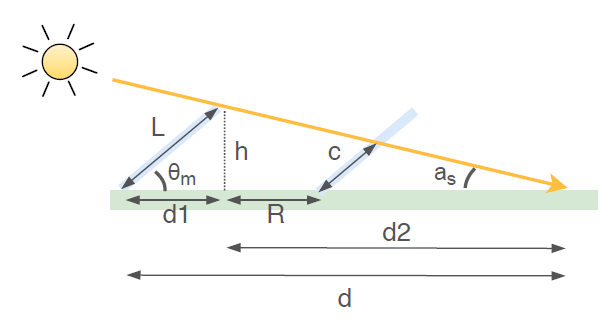
Fig. 1 - Side view of two modules showing a sunbeam casting a shadow on the module in the second row. The term coverage refers to shading length 𝑐.
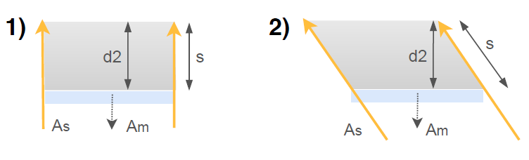
Fig. 2 - Two top views of a sunbeam (yellow) casting a shade (grey). Figure 1) shows the situation when the sun azimuth equals the module azimuth. Figure 2) shows the situation when this is not the case. Note that 𝑑2 in situation 1) equals 𝑠, the length of the shade seen from the top. 𝑑2 in this situation is referred to as 𝑑2(1).
When additionally considering the rowspace 𝑅 and the module tilt angle 𝜃𝑚, the final expression for the shaded length 𝑐(𝑡) on the module becomes:
𝑐(𝑡) =(𝑑2(𝑡) − 𝑅) ⋅ 𝑠𝑖𝑛(𝑎𝑠,2(𝑡)) / 𝑠𝑖𝑛(180 − 𝜃𝑚 − 𝑎𝑠,2(𝑡))
Another distinction made is regarding the module technology used and whether these contain bypass-diodes or not. It is assumed that mono and poly-crystalline silicon modules contain three bypass-diodes. For these modules, the calculated shading coverage 𝑐 is ceiled to the nearest third. In case of other (thin-film) technologies, the calculated, non-ceiled coverage values are used in further calculations.
Furthermore, the model automatically sets the shading coverage to zero in case of the several situations
where a module is not shaded:
- When the sun is behind the modules; However, this is not the case in a system with bifacial modules, but such modules are not yet implemented in the PVP.
- When the sun is below the horizon;
- When the shading brightness 𝑆𝐵 = 1;this requires 𝐻 = 0. This means that there is no direct light in comparison to diffuse light, as is the case in strong overcast conditions.
- When the tilt of the modules is zero: the modules are placed horizontally;
- When the length of the shade, 𝑑2(𝑡) is found to be equal to or less than the rowspace 𝑅;
- The first row does not suffer from mutual shading, but this is not incorporated in the PVP model yet.
DC power loss
For the calculations of the DC power including mutual shade loss, four cases are distinguished, also shown in Figure 1. For each case, the DC power is calculated by means of the corresponding equation:
- (A) landscape + c-Si modules --> 𝑃𝐷𝐶 = 𝑃𝑠𝑝𝑒𝑐𝑖𝑓𝑖𝑐 ⋅ 𝐴𝑎𝑐𝑡𝑖𝑣𝑒,𝑐𝑒𝑖𝑙𝑒𝑑
- (B) portrait + c-Si modules --> 𝑃𝐷𝐶 = 𝑃𝑠𝑝𝑒𝑐𝑖𝑓𝑖𝑐 ⋅ 𝑆𝐵 ⋅ 𝐴𝑚𝑜𝑑𝑢𝑙𝑒
- (C) landscape + other modules --> 𝑃𝐷𝐶 = 𝑃𝑠𝑝𝑒𝑐𝑖𝑓𝑖𝑐 ⋅ 𝑆𝐵 ⋅ 𝐴𝑚𝑜𝑑𝑢𝑙𝑒
- (D) portrait + other modules --> 𝑃𝑠𝑝𝑒𝑐𝑖𝑓𝑖𝑐 ⋅ 𝐴𝑎𝑐𝑡𝑖𝑣𝑒 + (𝑃𝑠𝑝𝑒𝑐𝑖𝑓𝑖𝑐 ⋅ 𝐴𝑠ℎ𝑎𝑑𝑒𝑑 ⋅ 𝑆𝐵)
Note that for cases (B) and (C) the same equation is used. It yields that 𝑃𝑠𝑝𝑒𝑐𝑖𝑓𝑖𝑐 = 𝐺𝑃𝑜𝐴,𝑓𝑖𝑛𝑎𝑙 ⋅ 𝜂𝐺,𝑇 ⋅ 𝜂𝑐𝑎𝑏𝑙𝑒,𝑀𝑀 in W/m2, which is the power the module produces per m2, after taking into account light capture losses, losses due to temperature and irradiance effects and the DC BoS components efficiency [1]. Furthermore, 𝐴𝑎𝑐𝑡𝑖𝑣𝑒 = 𝐴𝑚𝑜𝑑 ⋅ (1 − 𝑐𝑜𝑣𝑒𝑟𝑎𝑔𝑒) and 𝐴𝑠ℎ𝑎𝑑𝑒𝑑 = 𝐴𝑚𝑜𝑑 − 𝐴𝑎𝑐𝑡𝑖𝑣𝑒.
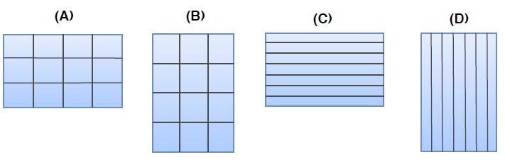
Fig. 1 - Mutual shading approach originating from four different cases: (A), landscape oriented cSi modules, (B) portrait oriented cSi modules, (C) landscape oriented thinfilm modules, and (D) portrait oriented thin-film modules.
As can be seen from the equations, assumptions are made for each case. First of all, c-Si modules are assumed to contain 3 bypass-diodes, dividing the module in 3 main strings. In landscape mode, every shaded string will produce zero power. In portrait mode, any shade will influence all strings, and the power output is then lowered by the shading brightness factor.
All other modules are treated as thin-film modules with one bypass-diode. In landscape mode, the DC power is calculated in the same way as in case (B). In portrait mode, both the shaded and unshaded areas contribute to the power production, albeit dependent on the shading brightness. In case of a fully dark shade, the power contribution of the shaded area is zero. From this power calculation, a ’mutual shading efficiency’ (𝜂𝑀𝑆) can be obtained, suitable to implement in the efficiency breakdown figure:
𝜂𝑀𝑆 = 𝐴𝑎𝑐𝑡𝑖𝑣𝑒/𝐴𝑚𝑜𝑑𝑢𝑙𝑒
𝜂𝑀𝑆 = 𝑆𝐵
𝜂𝑀𝑆 = (𝐴𝑎𝑐𝑡𝑖𝑣𝑒 + 𝑆𝐵 ⋅ 𝐴𝑠ℎ𝑎𝑑𝑒𝑑)/𝐴𝑚𝑜𝑑𝑢𝑙𝑒
Efficiency breakdown
The PVP model displays a summary of the calculated power losses happening in the designed PV system. The losses are visualized in a efficiency breakdown chart showing the system efficiency over the current day. This chart combines the calculated light capture losses, BoS losses and PV conversion losses. The chart also incorporates an estimate of the material dependent losses related to the theoretical efficiency limit (thermalization, non-absorption, and bandgap utilization [1]) and a fourth photovoltaic conversion loss called ‘opto-electrical loss’, that is calculated as the difference between the theoretical efficiency limit and the STC efficiency of the specific module [2]. This chart aims to provide insight to users about the dominant loss factors a a PV system and how these are composed.
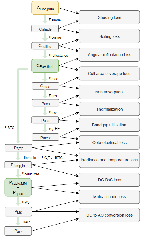
Fig. 1 - Flowchart of the efficiency breakdown calculations in [W/m2], including mutual shade loss, modelled as a DC power loss. It shows that the opto-electrical loss is calculated as the difference between 𝑃𝑆𝑇𝐶 and 𝑃𝑡ℎ𝑒𝑜𝑟.
[2] A. Ingenito, O. Isabella, S. Solntsev, and M. Zeman, “Accurate opto-electrical 5 modeling of multi-crystalline silicon wafer-based solar cells,” Sol. Energy Mater. Sol. 6 Cells, vol. 123, pp. 17–29, 2014.
Load & Sizing
The user input possibilities lead to two main modelling situations, that also can be combined:
- (1) The number of modules is (indirectly) specified by user and the area is unknown.
- (2) The area is specified by the user and the number of modules is unknown.
- (1+2) The number of modules is (indirectly) specified AND the area sides are specified.
Where we will call (1): ‘Modules to area’, and (2): ‘Area to modules’, both geometrical functions to calculate size-related parameters. These geometrical calculations strongly depend on the desired setup of your PV modules: the rowspace, tilt, azimuth and landscape/portrait orientation of the modules. For an east-west setup, the model also slightly changes. Details are found in [1].
Area types & array layout
Regarding the multiple possibilities of the size-input, a distinction between three 'types' of areas is made: (1) Available area: The actual available area as specified by the user by means of area sides. (2) Required area: The required area for a PV system with a number of modules based on the yearly load. (3) Desired area: The area obtained from specifying a desired number of modules by means of the size options ’number of modules’ or ’installed capacity’.
This distinction is important when displaying the system size results to the user, but also for ensuring a clear modelling structure. Depending on the user input, the corresponding areas should be determined, as shown in Figure 1. When there is more than one area type to be determined, only one of them should determine the final array layout displayed to the user. The ’array layout’ column states what parameters should serve as input for the array layout calculations.
Fig. 1 - Treediagram that shows which area types need to be determined depending on the load and size input options. The last column states what serves as the input for the array layout calculations. ”NM” stands for number of modules, ”IC” for installed capacity, ”RFA” for roof/field area, ”PP” for percentage of province and ”YE” for yearly electricity use. [1]
The ‘PV array layout’ model calculates one possible combination of how many PV modules are placed in a row and how many rows there are.
This layout is calculated from your size- and setup-related input. The layout is used for the calculations of the final dimensions of your PV system, as described in detail in [1].
In the PVP model, this array layout generally does not influence the performance calculations: it does not matter whether you have an 4x3 layout or an 2x6 layout, as long as the number of modules stays the same. However, in case of an east-west setup it depends how many of these modules are facing east and how many west. In this case, the layout could slightly influence the performance calculations.
Load: energy balance
The approach for calculating the system size from the load is based on a gridconnected
system sizing method described in [1], chapter 20.4. It originates from the energy balance paradigm: the system
size is estimated in such a way that the produced energy and the consumed energy match over the
year.
𝑁𝑙𝑜𝑎𝑑 = ceil(𝐸Υ𝐿 ⋅ 𝑆𝐹 / 𝐴mod ⋅ ∫𝐺𝑀,𝑦𝑒𝑎𝑟(𝑡)𝜂(𝑡) d𝑡)
Here, 𝑁𝑙𝑜𝑎𝑑 is the estimated (ceiled) required number of modules, 𝐸Υ𝐿 the specified yearly electricity
use in Wh, 𝑆𝐹 a commonly used sizing factor of 1.1, 𝐴mod the area of one module and 𝜂(t) taken to be 𝜂𝑆𝑇𝐶. The expression ∫𝑦𝑒𝑎𝑟𝐺𝑀(𝑡)𝜂(𝑡) d𝑡 is the yearly (potential) DC energy per m2 produced by one module, in Wh/m2.
An addition made for this sizing approach is the implementation of a ’percentage of load’ factor (0-1). By
specifiying this factor, the user can define what percentage of the load they want to be covered. 𝐿𝑜𝑎𝑑𝐹𝑎𝑐𝑡𝑜𝑟 = 1, means that the intention is to cover
100% of the yearly electricity use.
Minimal rowspace calculation
The user can choose between specifying a certain rowspace or letting the model calculate a minimal rowspace. This minimal rowspace is the rowspace needed to have (almost) no mutual shading loss during a year. It is determined as follows:
The rowspace should be such that no shading occurs for 5 hours during the shortest day of the year (21st of december). This means that during the rest of the year, the shading would be lower. A timeframe from 10AM-3PM is used. The first step is to calculate the azimuth and altitude of the sun at both 10AM and 3PM this day.This is done by using the same equations used for calculating the sun position for the meteorological databases, obtained from [1].
Then, the length of the casted shade is calculated for both hours, using the same approach as for the mutual shading coverage. For both hours, it is checked whether the sun is behind the modules. If this for example is the case at 10AM due to west-facing system, the shading length at 15PM, 𝑑2-15, is used to determine the minimum rowspace 𝑅. When at both 10AM and 15PM the sun is in front of the module, the shadowlengths for both times are compared and it then yields: 𝑅 = 𝑚𝑎𝑥(𝑑2-15, 𝑑2-10) [2].
In an EW setup, the approach is slightly different, since the sun will always be in front of either the west or the east facing modules. The rowspace is calculated by taking the maximum of the absolute values of the calculated shadowlenghts and compensating for the different definition of rowspace as seen in Figure 1, meaning that 𝑅 = 𝑚𝑎𝑥(𝑑2-15, 𝑑2-10) - 𝑑1. Additionally, a check is performed to ensure that when 𝑅 ≤ 𝑑1, the rowspace is set to zero.
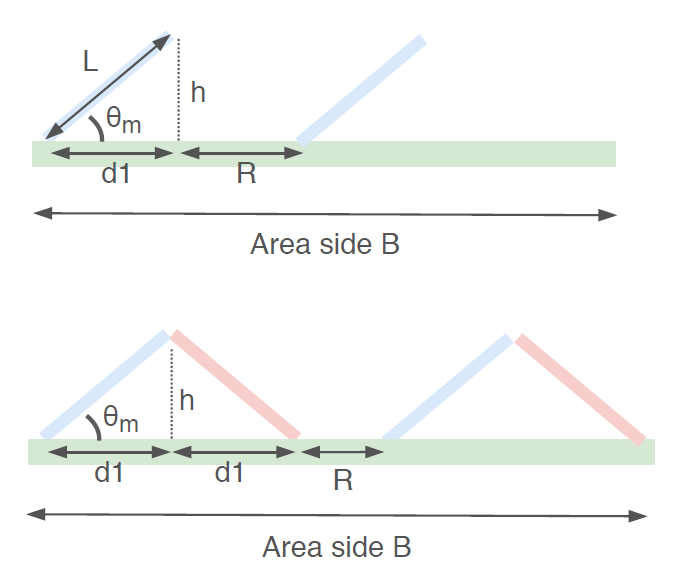
Fig. 1 - Two sideviews showing area side B for a normal configuration (left) and for an EW configuration (right).
Economic model
The economic calculations depend on the economic input (also related to the user's system choices): (1) PV system lifetime, (2) the initial investment cost, (3) the annual operation and maintenance (O&M) cost, (4) the annual energy production (which includes a panel degradation factor leading to decreased production over time), (5) the annual revenue (depending on electricity prices and regulations), and (6) the discount rate.
This input is used to calculate four economic indicators that are relevant for PV systems to determine whether the investment is worthwhile: the net present value (NPV), the (discounted) payback period ((D)PBP), the compound annual growth rate (CAGR), and the levelized cost of electricity (LCoE). Each indicator can highlight a different aspect of the investment.
Economic input
For the calculations we need: (1) PV system lifetime, (2) the initial investment cost, (3) the annual operation and maintenance (O&M) cost, (4) the annual energy production (which includes a panel degradation factor leading to decreased production over time), (5) the annual revenue (depending on electricity prices and regulations), and (6) the discount rate. Table 1 gives an overview of the how each input is obtained.
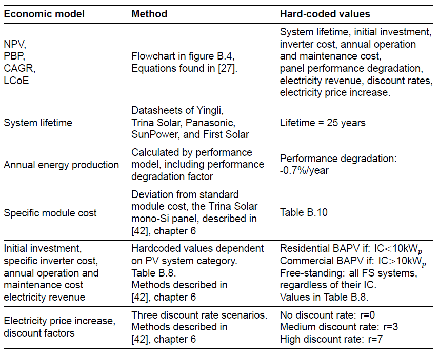
Tab. 1 - Summary of approach for economic model [4].
For input (2)-(5), to deal with economies of scale, a division of PV systems into three PV system categories was done, comparable to the approach used by the Nationaal Solar Trendrapport, Solar Bankability and an economic study of the International Energy Agency [1], [2], [3]. Specific inverter cost are calculated by downscaling the average value depending on system type with Inverter Sizing Factor of the designed system. Table 2 summarizes the category-dependent values used for the economic calculations.
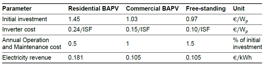
Tab. 2 - Economic parameters dependent on system category [4].
The standard module cost is assumed to be equal to the Trina Solar mono c-Si panel. If an alternative module is chosen, the difference between this module cost and the Trina mono c-Si panel cost is added to the standard total system cost applied for the PV system category.
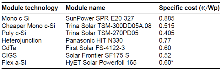
Tab. 3 - Overview of PV modules and specific costs as found in the PVP 2.0 report [5]. *The cost of the flexible a-Si module is not known and therefore assumed to be equal to the CdTe module price.
[2] M. Richter C. Tjengdrawira and I. Theologitis. Best practice guidelines for pv cost calculation accounting for technical risks and assumptions in pv lcoe, 2016.
[3] IEA. Projected costs of generating electricity 2015 edition, 2015.
[4] The Dutch PV Portal 3.0, M. Klement, 2019.
[5] Veikko Schepel. The dutch pv portal 2.0. Thesis report, Delft University of Technology, 2018.
Economic indicators
To provide a scientifically based profitability analysis, four economic indicators are calculated [1]:
The net present value (NPV, in €) of the PV system. The NPV is the current value of the profit (or loss) made over the investment lifetime.
The second indicator, the payback period (PBP, in years) indicates the amount of time it will take for the total profit to outweigh the initial investment.
The compound annual growth rate (CAGR, in %) indicates the average annual interest made over the total investment. The CAGR of the PV system can be compared with the standard interest rate expected by website users.
The fourth and final indicator is levelized 1 cost of electricity (LCoE, in €/kWh). The LCoE represents the amount of money it costs to produce one kWh of electricity. The LCoE is an indicator through which the cost-competitiveness of PV versus other energy generation technologies can be compared.